uvnote Integration Test Report

import numpy as np
import pandas as pd

# Set seed for reproducibility
np.random.seed(42)

# Generate sample data
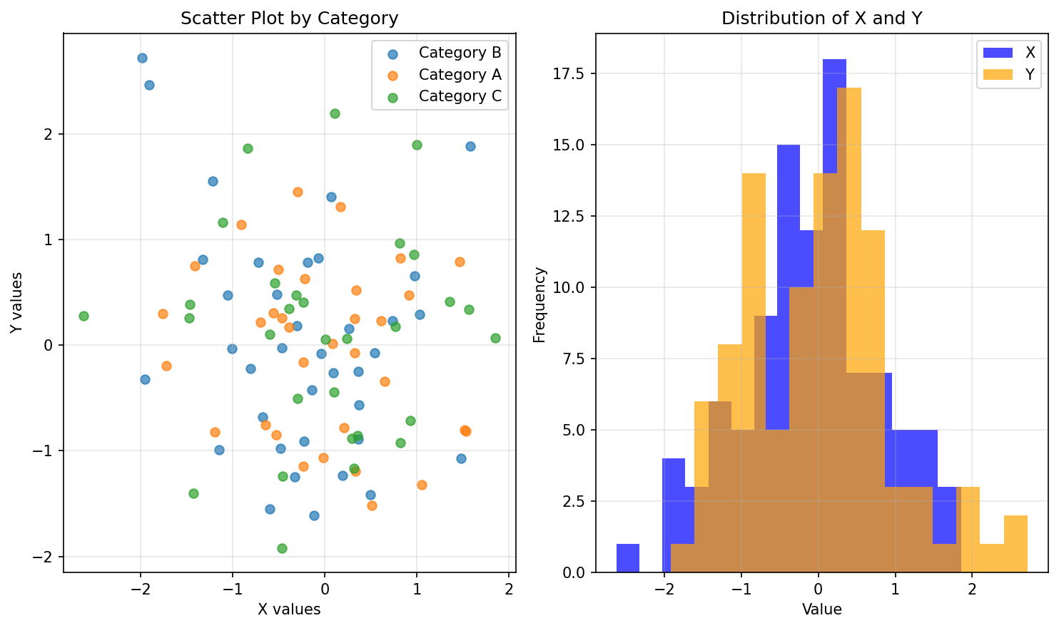
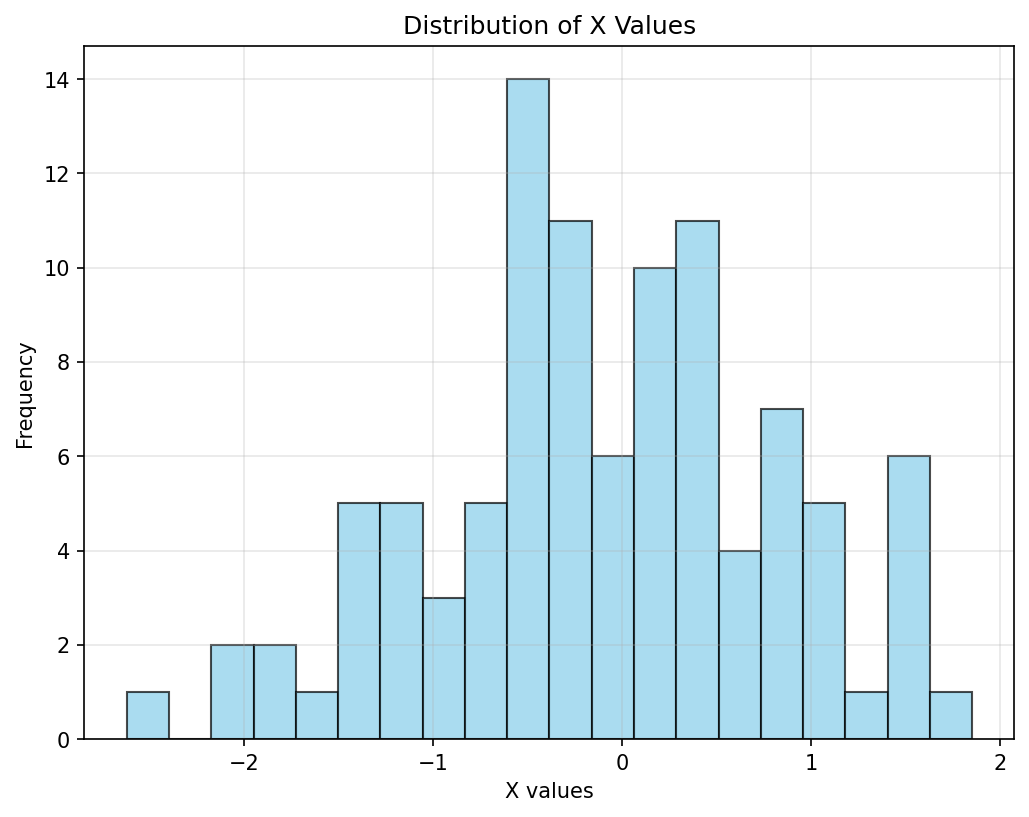
n_points = 100
data = pd.DataFrame({
    'x': np.random.normal(0, 1, n_points),
    'y': np.random.normal(0, 1, n_points),
    'category': np.random.choice(['A', 'B', 'C'], n_points)
})

print(f"Generated {len(data)} data points")
print("\nFirst 5 rows:")
print(data.head())

print(f"\nData types:")
print(data.dtypes)

import numpy as np
import pandas as pd

# Recreate the same data with same seed
np.random.seed(42)
n_points = 100
data = pd.DataFrame({
    'x': np.random.normal(0, 1, n_points),
    'y': np.random.normal(0, 1, n_points),
    'category': np.random.choice(['A', 'B', 'C'], n_points)
})

# Calculate basic statistics
stats = data.describe()
print("Descriptive Statistics:")
print(stats)

# Category counts
print("\nCategory distribution:")
print(data['category'].value_counts())

# Correlation
correlation = data[['x', 'y']].corr()
print(f"\nCorrelation between x and y: {correlation.iloc[0,1]:.3f}")

import matplotlib.pyplot as plt
import pandas as pd
import numpy as np

# Recreate the same data with same seed
np.random.seed(42)
n_points = 100
data = pd.DataFrame({
    'x': np.random.normal(0, 1, n_points),
    'y': np.random.normal(0, 1, n_points),
    'category': np.random.choice(['A', 'B', 'C'], n_points)
})

# Create scatter plot
plt.figure(figsize=(10, 6))

# Subplot 1: Scatter plot by category
plt.subplot(1, 2, 1)
for cat in data['category'].unique():
    cat_data = data[data['category'] == cat]
    plt.scatter(cat_data['x'], cat_data['y'], label=f'Category {cat}', alpha=0.7)

plt.xlabel('X values')
plt.ylabel('Y values') 
plt.title('Scatter Plot by Category')
plt.legend()
plt.grid(True, alpha=0.3)

# Subplot 2: Histogram
plt.subplot(1, 2, 2)
plt.hist(data['x'], bins=15, alpha=0.7, label='X', color='blue')
plt.hist(data['y'], bins=15, alpha=0.7, label='Y', color='orange')
plt.xlabel('Value')
plt.ylabel('Frequency')
plt.title('Distribution of X and Y')
plt.legend()
plt.grid(True, alpha=0.3)

plt.tight_layout()
plt.savefig('scatter_plot.png', dpi=150, bbox_inches='tight')
plt.close()

# Create individual histogram
plt.figure(figsize=(8, 6))
plt.hist(data['x'], bins=20, alpha=0.7, color='skyblue', edgecolor='black')
plt.xlabel('X values')
plt.ylabel('Frequency')
plt.title('Distribution of X Values')
plt.grid(True, alpha=0.3)
plt.savefig('histogram.png', dpi=150, bbox_inches='tight')
plt.close()

print("Plots saved successfully!")
print("- scatter_plot.png: Combined scatter plot and distribution")
print("- histogram.png: X value distribution")

import pandas as pd
import numpy as np

# Recreate the same data with same seed
np.random.seed(42)
n_points = 100
data = pd.DataFrame({
    'x': np.random.normal(0, 1, n_points),
    'y': np.random.normal(0, 1, n_points),
    'category': np.random.choice(['A', 'B', 'C'], n_points)
})

# Save data to CSV
data.to_csv('data.csv', index=False)
print("Data saved to data.csv")

# Create summary file
with open('summary.txt', 'w') as f:
    f.write("Data Summary Report\n")
    f.write("==================\n\n")
    f.write(f"Total data points: {len(data)}\n")
    f.write(f"Columns: {list(data.columns)}\n")
    f.write(f"X range: {data['x'].min():.3f} to {data['x'].max():.3f}\n")
    f.write(f"Y range: {data['y'].min():.3f} to {data['y'].max():.3f}\n")
    f.write(f"Categories: {sorted(data['category'].unique())}\n")

print("Summary saved to summary.txt")

import os
import pandas as pd

# Discover the upstream artifact directory from env
data_dir = os.environ.get('UVNOTE_INPUT_SAVE_DATA', '.')
csv_path = os.path.join(data_dir, 'data.csv')

df = pd.read_csv(csv_path)
print(f"Dependent cell read {len(df)} rows from save_data/data.csv")
print(f"x mean: {df['x'].mean():.3f}, y mean: {df['y'].mean():.3f}")